Bootstrapping Examples in R

What is Bootstrapping?

Bootstrapping is a procedure for estimating the distribution of an estimator by resampling (often with replacement) from the data or from a fitted model.

It assigns measures of accuracy (bias, variance, confidence intervals, prediction error) to sample estimates and allows estimation of the sampling distribution of almost any statistic using simulation.

I use rnorm function (randomize + normal distribution) to generate a practice set of data.

Fit model

set.seed(123)

x <- rnorm(50, mean = 10, sd = 2)
n <- length(x)

mu_hat <- mean(x)
sd_hat <- sd(x)

Run bootstrap

B <- 1000
mu_boot <- numeric(B)

for (b in 1:B) {
  x_star <- rnorm(n, mean = mu_hat, sd = sd_hat)
  mu_boot[b] <- mean(x_star)
}

results

boot_mean <- mean(mu_boot)
boot_se <- sd(mu_boot)
ci <- quantile(mu_boot, c(0.025, 0.975))

boot_mean

[1] 10.06563

boot_se

[1] 0.2470952

ci

     2.5%     97.5% 
 9.585642 10.531793 

Example for linear regression

set.seed(123)

n <- 100
x <- runif(n, 0, 10)
y <- 5 + 2 * x + rnorm(n, 0, 2)

Fit linear model

fit <- lm(y ~ x)
summary(fit)

Call:
lm(formula = y ~ x)

Residuals:
    Min      1Q  Median      3Q     Max 
-4.4759 -1.2265 -0.0395  1.1927  4.4345 

Coefficients:
            Estimate Std. Error t value Pr(>|t|)    
(Intercept)  4.98208    0.39211   12.71   <2e-16 ***
x            1.98203    0.06836   28.99   <2e-16 ***
---
Signif. codes:  0 '***' 0.001 '**' 0.01 '*' 0.05 '.' 0.1 ' ' 1

Residual standard error: 1.939 on 98 degrees of freedom
Multiple R-squared:  0.8956,    Adjusted R-squared:  0.8945 
F-statistic: 840.6 on 1 and 98 DF,  p-value: < 2.2e-16

Extract parameters

beta_hat <- coef(fit) 
sigma_hat <- summary(fit)$sigma

Bootstrap

B <- 1000
beta_boot <- matrix(NA, nrow = B, ncol = length(beta_hat))

for (b in 1:B) {
  y_star <- beta_hat[1] + beta_hat[2] * x + rnorm(n, 0, sigma_hat)
  fit_star <- lm(y_star ~ x)
  beta_boot[b, ] <- coef(fit_star)
}

Results

boot_means <- colMeans(beta_boot)
boot_ses <- apply(beta_boot, 2, sd)
boot_ci <- apply(beta_boot, 2, quantile, probs = c(0.025, 0.975))

boot_means

[1] 4.956659 1.987527

boot_ses

[1] 0.39379308 0.06913355

boot_ci

          [,1]     [,2]
2.5%  4.226149 1.858384
97.5% 5.727671 2.115856

Example for logistic regression

Generate data using runif (randomize uniform distribution)

set.seed(123)

n <- 200
x <- runif(n, 0, 10)

beta0 <- -2
beta1 <- 0.5

p <- 1 / (1 + exp(-(beta0 + beta1 * x)))
y <- rbinom(n, 1, p)

data <- data.frame(y = y, x = x)

fit <- glm(y ~ x,
           family = binomial(link = "logit"),
           data = data)

summary(fit)

Call:
glm(formula = y ~ x, family = binomial(link = "logit"), data = data)

Coefficients:
            Estimate Std. Error z value Pr(>|z|)    
(Intercept) -1.77952    0.36534  -4.871 1.11e-06 ***
x            0.47483    0.07425   6.395 1.61e-10 ***
---
Signif. codes:  0 '***' 0.001 '**' 0.01 '*' 0.05 '.' 0.1 ' ' 1

(Dispersion parameter for binomial family taken to be 1)

    Null deviance: 267.50  on 199  degrees of freedom
Residual deviance: 210.62  on 198  degrees of freedom
AIC: 214.62

Number of Fisher Scoring iterations: 4

Extract estimated parameters

beta_hat <- coef(fit)

B <- 1000
beta_boot <- matrix(NA, nrow = B, ncol = length(beta_hat))


for (b in 1:B) {
  p_hat <- 1 / (1 + exp(-(beta_hat[1] + beta_hat[2] * x)))
  y_star <- rbinom(n, 1, p_hat)
  
  fit_star <- glm(y_star ~ x,
                  family = binomial(link = "logit"))
  
  beta_boot[b, ] <- coef(fit_star)
}

colnames(beta_boot) <- names(beta_hat)

Results

boot_means <- colMeans(beta_boot)
boot_ses <- apply(beta_boot, 2, sd)
boot_ci <- apply(beta_boot, 2, quantile, probs = c(0.025, 0.975))

results <- data.frame(
  Estimate = beta_hat,
  BootMean = boot_means,
  BootSE = boot_ses,
  CI_lower = boot_ci[1, ],
  CI_upper = boot_ci[2, ]
)

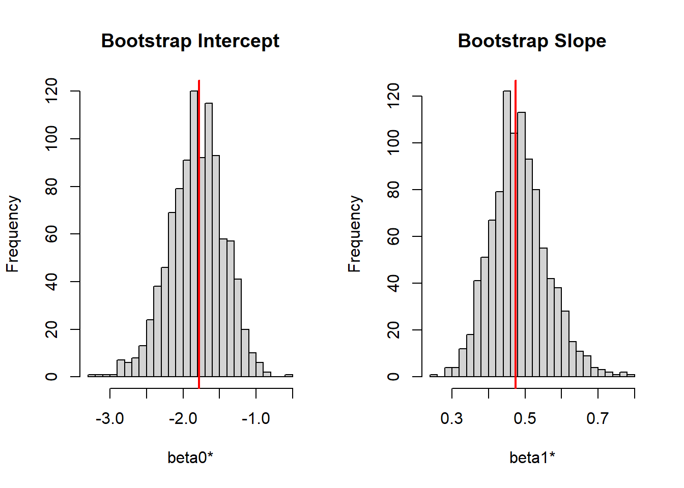
print(results)

             Estimate   BootMean     BootSE   CI_lower  CI_upper
(Intercept) -1.779518 -1.8127758 0.37463075 -2.5968318 -1.133648
x            0.474827  0.4839984 0.07756396  0.3501373  0.649960

lets graph both intercept and slope using histogram

par(mfrow = c(1, 2))

hist(beta_boot[,1],
     main = "Bootstrap Intercept",
     xlab = "beta0*",
     breaks = 30)
abline(v = beta_hat[1], col = "red", lwd = 2)

hist(beta_boot[,2],
     main = "Bootstrap Slope",
     xlab = "beta1*",
     breaks = 30)
abline(v = beta_hat[2], col = "red", lwd = 2)